How (not) to cosine. Part 1

To cosine or not to cosine

There was a recent reddit post about implementing cos(x) from scratch in C.

In which the author explored two different approaches to implementing (an approximate) cosine function, which can serve as a great example to show why “textbook math”¹ approaches to numerical algorithms can often fall short (or alternatively: why the whole field of numerics exists).

This post is not intended to poke fun at the author, but rather to show some numerical techniques that are usually not taught in normal algebra or calculus classes. Note that having a basic understanding of calculus is all that’s required to follow this post, you’re not expected to have studied any numerics related topics before.

Why Mr. Taylor isn’t your friend

When faced with the problem of implementing a function to calculate cos(x) a natural idea might be to use a Taylor series. In fact the Taylor series for cos(x) follows a rather nice pattern:

cos(x) = 1 - x^2/2! + x^4/4! - x^6/6! + ...

The ... here indicates that there are actually infinitely many terms to the series. From this we can obtain a truncated Taylor series by using just a finite number of terms and discarding the rest:

cos(x) ≈ 1 - x^2/2! + x^4/4! - x^6/6!

And while Taylor series are a great tool for proofs in calculus classes, using a truncated Taylor series to approximate an analytic function will rarely yield great results.

To understand why, we have to take a closer look at how polynomial approximations work. First of all even though our original Taylor series might “converge everywhere”, our truncated Taylor series will actually have a finite interval on which it approximates the desired function well. Outside of that interval it will quickly diverge to positive or negative infinity.

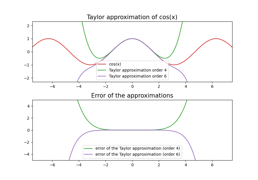
One striking feature in the error plot is the monotonicity: the further away from x = 0 we get, the larger the error. This is a problem…

Polynomials want to be curvy

For a given interval we care about the maximum error of our approximation. To improve this, we can obviously just increase the order of the polynomial (i.e. use more terms of the Taylor approximation). But this means that our function takes longer and longer to compute. So if we have decided on some number of terms that we deem “sufficiently few to be fast enough to compute”, we want to find a polynomial with that many terms which will have the smallest maximum error over our interval.².

And here we encounter an interesting property of polynomials: They want to be curvy! The error of our Taylor polynomial grows much faster than necessary due to the fact that its error is not “allowed to oscillate”. It grows monotonically, meaning that for any interval we choose it will always take its maximum value at on of the interval’s end points. This indicates an interesting property of Taylor approximations: They are “well behaved” close to one point and have a monotonically growing error. We can choose this point however we want, but we can only choose a single point.

Fitting a polynomial to some arbitrary function is a bit like trying to force an elastic pizza dough into a specific shape: We can use our hands to fix it in some places, but not everywhere. We can obviously get some friends to help us (which would be analogous to using a polynomial of higher degree), but for a given number of hands to fix certain points in place, there will be others, that deviate from the desired shape. So we have to be clever about where exactly we pull on the dough to ensure the best fit.

So if we imagine a sort of “accuracy budget” we can work with, then by using a Taylor approximation we exhausted it all to keep anything close to one point accurate. But there are in fact smarter ways to make use of our “accuracy budget” by allowing the error to become larger in some places in order for it to decrease in others. In particular our current error is either always positive or always negative, but from an accuracy standpoint we do not care about the sign of the error, only its magnitude.

So how do we design a polynomial that minimizes the maximum error over an interval? We evaluate our function at n points in the interval and then fit a polynomial of degree n-1 through those points. Here we can choose whichever points we want (e.g. we could just space out our n points evenly across the interval, group them all in the center etc.). As it turns out, choosing the so called “Chebyshev nodes”³ over our interval will often yield near optimal results.

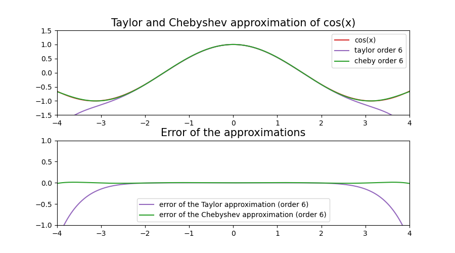
Now that’s a huge difference! Somewhere at around x = 2.5 the error of the Taylor approximation “explodes” whereas the Chebyshev approximation follows the original function over the whole interval, even though it has the same order!

If we zoom in, we discover something interesting….

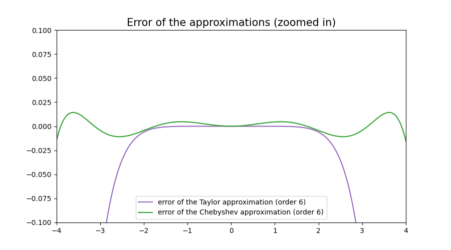
The error of the Chebyshev approximation oscillates over the whole interval. By “allowing” the polynomial to be “more curvy”, we got a much better maximum error overall.

Range reduction (how much cosine do you need anyway?)

When designing a numerical approximation, we should always try to make the interval over which the approximation has to be correct as small as possible. For cos(x) there are a few obvious way in which this can be done.

First of all we know that cos(x) = cos(-x), which lets us disregard all negative values if we just compute the absolute value of x:

float my_cos(float x){
    x = abs(x);         // cos(-x) == cos(x)
    float result = .... // magic
    return result;
}

Next we know that cos(x) is a periodic function that repeats at every multiple of 2π. Which in turn means that if we are able to find the largest multiple of 2π less than x, we can subtract that from x and calculate cos of the result:

float my_cos(float x){
    x = abs(x);         //      cos(-x) == cos(x)
    x = fmod(x, 2*pi);  // cos(x + 2pi) == cos(x)
    float result = .... // magic
    return result;
}

But that’s not all! If our goal is to restrict the interval over which our approximation has to be good, we can actually do a bit more:

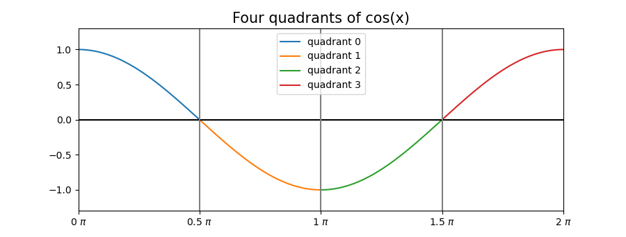
The first quadrant is mirrored and repeated for three more times. So our approximation can be reduced to the interval [0, pi/2] if we do some clever mirroring:

if(x > 3*pi/2){                 // quadrant 3
    x = 3*pi/2 - x;             // mirror vertically
}
... //similar mirroring for quadrants 1 and 2

Reducing our interval of interest to [0, pi/2] should improve our error, because a smaller interval means that we can make more efficient use of our “accuracy budget”. We will also include a fifth order Chebyshev approximation for comparison:

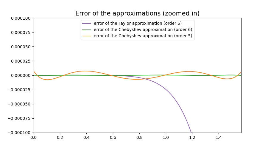
That’s another serious improvement. The maximum error of our sixth order Chebyshev approximation is now well below 10^-5, in fact we got it down to 4.3*10^-7(!)

And the error of the fifth order Chebyshev approximation manages an error less than 7.8*10^-6,

whereas the maximum error of the Taylor polynomial sits firmly at 8.9*10^-4

With the construction of our polynomial out of they way, we’ll focus on the actual implementation in the next part.

---

1. “textbook” here refers to typical calculus textbooks. Numerics textbooks obviously do exist and teach the proper techniques, but they often aren’t part of a typical university math course. ↩

2. In real world applications this is often done the other way around: we decide on a maximum error bound and then find the lowest order polynomial that achieves said goal. ↩

3. Chebyshev Nodes on wikipedia ↩